In the wake of the collapse of the credit and housing markets, much attention has been focused on traditional mortgage and mortgage-backed-security performance. However, despite the reduction in available credit, one mortgage market has continued its steady growth through the financial turmoil: the reverse-mortgage market.
A reverse mortgage allows a homeowner to withdraw equity from a home in various forms, to be repaid upon the sale of the property. Aside from origination and servicing-fee income, an issuer of reverse mortgages profits from the transaction when the sale of the property is sufficient to cover the amount of equity withdrawn plus interest and fees. Reverse mortgages are nonrecourse loans (i.e., the lender has no recourse beyond the property in question), so losses occur if the home is sold for less than the amount owed. In order to mitigate this risk (generally referred to as crossover risk), the most commonly originated loans are Home Equity Conversion Mortgages (HECMs), in which the lender is insured against crossover risk by the United States government.
The U.S. Department of Housing and Urban Development (HUD) endorsed its first HECM loan in 1989 and has endorsed over 525,000 loans since, with about 400,000 of those endorsements occurring between 2004 and 2008. HECMs account for nearly 90% of the entire reverse-mortgage market, meaning that nearly all of the reverse-mortgage risk lies with the U.S. federal government. This raises the question, what happens to the HECM portfolio when the value of the average U.S. home falls 30%, 40%, or even 50% over a relatively short period of time?
What is an HECM mortgage?
HECM loans are reverse mortgages insured by HUD. When HECM loans are originated, the borrower receives payments in the form of lump sums, term/tenure payments, or lines of credit, and the borrower does not have to make any repayments on the loan prior to a maturity event (defined as the death of the borrower or permanent move-out from the property). HECM loans are non-recourse loans, meaning that the lender cannot seek restitution in excess of the value of the property at loan maturity. The insurance that HUD provides indemnifies reverse-mortgage issuers—approved Federal Housing Administration (FHA) lenders—in the event that the loan balance exceeds the proceeds from the sale of the property at maturity. HECMs, the only reverse mortgages insured by the U.S. federal government, were designed to be a self-funding (zero-subsidy) program. In order to fund the HECM insurance program, HUD charges an initial mortgage insurance premium of 2% of the value of the home (subject to FHA lending limits) plus an annual renewal fee of 0.5%. Using this premium structure, HUD developed the principal limit factors that mandate the amount of money borrowers may be eligible to receive, subject to various criteria. These criteria include, among other things, minimum age requirements, loan size limits, and primary residence status.
Until September 2009, the principal limit factors governing the amount of money available to HECM borrowers had remained unchanged from the program’s inception in 1989. However, on September 23, 2009, HUD issued Mortgagee Letter 09-34, which stated that the amount of money available to HECM borrowers was going to be reduced.
This action was taken as a result of an indicated required-credit subsidy for the HECM program during HUD’s annual budget review. Because the HECM program is mandated to be a zero-subsidy program, HUD was faced with the options of discontinuing the program or reshaping the program to comply with its original mission. It is safe to assume that these revisions to the HECM program are a direct result of the pressures facing the current economy. Following this premise, we have framed the results of our analysis around the change in the principal limit factors.
What are the risk-drivers of HECM?
HECM loans do not allow borrowers access to 100% of the equity in their homes; rather, borrowers are allowed access to only a portion of the equity in their homes, depending on the borrower and economic criteria. At the outset of the HECM program in 1989, HUD calculated the principal limit factors that dictated the amount of money a borrower could access, based on long-term economic and loan termination assumptions. The principal limit factors were set by determining the appropriate loan-to-value (LTV) ratio such that the insurance premium would cover expected future losses.
The creation of the HECM principal limit factors required the consideration of the three key risk-drivers of crossover risk for HECM loans:
- interest-rate risk
- loan termination rates
- home price appreciation
Loan interest is capitalized in the loan balance over time, so the amount of money owed varies directly with the interest rate applied. Crossover risk varies proportionally with current interest-rate levels. Given that HECM loans can be adjustable-rate mortgages (ARMs), HECM used an expected interest rate over the life of each loan in determining the principal limit factor. If interest rates turn out to be significantly higher than the expected interest rate, the loan will accumulate at a faster rate than expected and could result in a potentially greater crossover risk than indicated by the premium charged.
Given that HECMs become due when borrowers either die or move out of their houses, the second key risk-driver for HECM loans is the loan termination date. In generating principal limit factors, HUD assumed that loan terminations would occur consistently with a fixed multiple of rates indicated in published actuarial mortality tables. Using these termination rates, HUD estimated principal limit factors for borrowers ranging in age from 62 to 95 and the expected interest rate. If HUD has overestimated the termination rates, then HECMs will accumulate for a longer period than expected and result in greater crossover risk than indicated by the premium charged.
The final risk faced by HECM is the impact of home price appreciation (HPA) on the properties that collateralize the loans. If HPA is greater than anticipated, properties collateralizing loans will be worth more, increasing the likelihood of paying off the entire loan balance. Conversely, crossover risk increases to the extent that houses appreciate less than anticipated. In generating the principal limit factors, HUD postulated that home prices would appreciate at 4% per year, consistent with historical experience (see Figure 1). To the extent that HPA paths are significantly less than 4% per year, the HECM portfolio could face greater crossover risk than indicated by the premium charged.
The principal limit factors were calculated to vary by borrower age and the current interest-rate environment. Assuming that the expected rate at loan origination is truly reflective of the future interest-rate path, this means that the major risks to HECM principal limit pricing are the termination rates and HPA. Recent research has indicated that the termination assumptions used by HUD in generating HECM principal limits were conservative, particularly at higher ages. This paper is not intended to address those considerations; rather, the intent of this paper is to investigate the impact of the recent bursting of the housing bubble on the HECM principal limits.
In order to examine the impact of current HECM originations, we developed three HPA scenarios to run through an HECM pricing model. The model is based on the paper by Edward J. Szymanoski, Jr., "Risk and the Home Equity Conversion Mortgage." The model discussed in the paper (which is a re-creation of the methodology used to describe HECM pricing) has been reproduced and adjusted here to allow for more dynamic HPA paths. The three paths used to test the effect of the housing-bubble burst on the HECM portfolio are as follows (also see Figure 1):
Scenario 1: Peak-to-trough decline of 30% followed by 4% growth thereafter
This scenario assumes the housing bubble was a one-time downward shock to the long-term average growth of housing prices; once the market comes back, home price trends will return to historical growth.
Scenario 2: Peak-to-trough decline of 45% followed by 2% growth thereafter
This scenario assumes a prolonged decline in home prices followed by a prolonged period of slow growth in housing prices; this scenario is similar (although more optimistic) to the actual home price growth in Japan from the 1990s to 2009.
Scenario 3: Average of Scenario 1 and Scenario 2
The above scenarios were selected to represent reasonable home-price forecasts for the HECM portfolio. The HECM portfolio has a significant amount of exposure to loans issued in California and Florida (35% by count and 42% by dollar exposure); these two states have experienced some of the most severe home-price declines in the nation, with home prices already declining 35% on average in these two states. In addition, these scenarios are consistent with current economic forecasts of future home prices.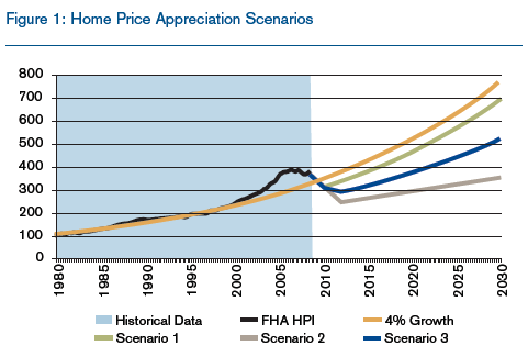
Analysis of the impact of home price appreciation on one HECM portfolio...
We will use a single-loan example to test the impact of the above three scenarios on the HECM portfolio. The single loan will have the following characteristics:
Borrower age: 75
Expected interest rate: 10%
Principal limit factor (Before Oct. 1, 2009): 41.60%
Principal limit factor (After Oct. 1, 2009): 37.40%
Initial home value: $100,000
The impact of the HPA path can be measured in a variety of ways. The first metric we show is the required subsidy for the loan as determined by the present value of expected loss less the present value of expected premium. Note that a negative value is equivalent to a profit, because the present value of losses is less than the present value of premiums, and a positive value is equivalent to a loss, as the present value of losses exceeds the present value of premiums. Figure 2 depicts the estimated required subsidy for the above loan for origination years 1989 to 2020.
In this figure, the dotted lines represent the estimated required subsidy, assuming the principal limit factors in effect prior to October 1, 2009; the solid lines reflect the estimated subsidy, assuming the principal limit factors in effect subsequent to the revision.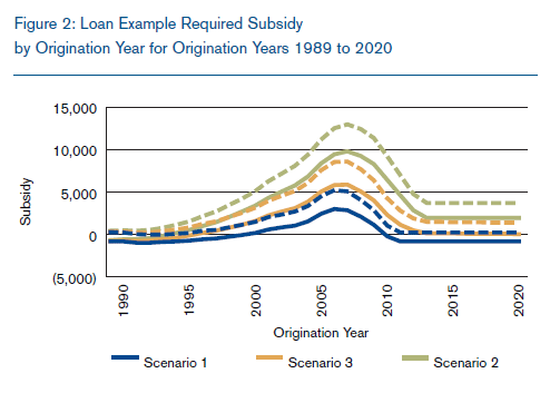
The y-axis of the above chart represents the subsidy for the loan, given the HPA scenario, expected interest rate of 10%, and termination rates consistent with those originally used in generating the HECM principal limits. The x-axis represents the origination year. For example (and looking first at the original HECM principal limits; i.e., the dotted lines), the above loan issued in 1992 under Scenario 1 has a small estimated negative subsidy of -$286, indicating a profit to HUD; the above loan originated in 2006 requires an estimated subsidy of about $4,500 for Scenario 1, $8,000 for Scenario 3, and $12,500 for Scenario 2. For loans issued after 2011, when HPA is assumed to return to 4% for Scenario 1, the loan is assumed to break even and return to a zero-subsidy program using the original principal limits. The chart demonstrates the impact of HPA on the required subsidy of an HECM loan. Depending on the origination year of the loan, the required subsidy of the loan shifted from a slightly negative subsidy for loans issued in the early 1990s to a required subsidy of about $12,500 per loan in the worst-case scenario. This result is consistent with the decline in home-price-scenario results from Bishop and Shan’s 2008 analysis, "Reverse Mortgages: A Closer Look at HECM."
As one would expect, the revision to the principal limit factors decreases the estimated subsidy for all vintages in each scenario. In the worst years (2006 and 2007), the reduced factors have the impact of reducing the implied subsidy by $2,000 to $3,000, depending on the scenario. It is also interesting to note that the revised factors indicate roughly a zero-subsidy in years 2013 and subsequent in Scenario 3. This indicates that the new factors are consistent with those which would have been calculated at program inception if the HPA assumption employed had been 3% annually instead of 4%.
Another way to quantify the impact of these HPA paths is to change the principal limit factors such that the same premium structure would result in a zero-subsidy program each year. In other words, what percent of equity could HUD allow HECM borrowers to tap into without generating the need for a taxpayer subsidy, given these HPA paths? The graph in Figure 3 shows the indicated principal limit factors for the borrower referenced above in the three scenarios.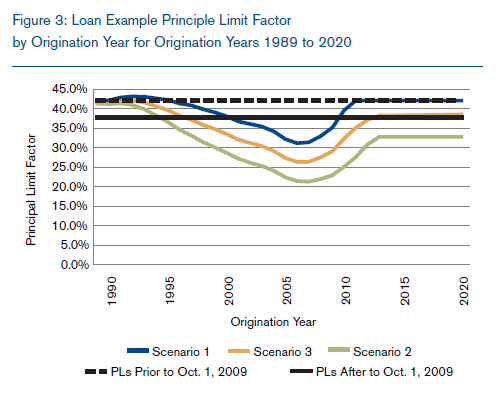
As shown in Figure 3, the principal limits generating zero-subsidy for HECM loans decrease significantly as the housing market approaches its peak in 2006 and 2007. The indicated principal limit at the peak of the market varies from roughly one-half to three-quarters of the actual principal limit offered, depending on the economic scenario modeled. As the forecast of house prices nears its bottom, the estimated principal limits begin to return to the levels originally indicated by HECM pricing. You can once again see that the principal limit factors subsequent to the revision are consistent with those indicated in Scenario 3 for 2013 and the years beyond.
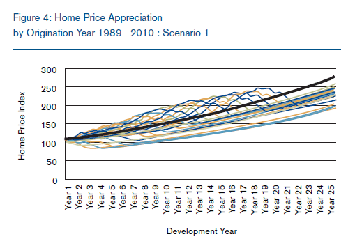
Note that in Figures 2 and 3 a significant deviation from the assumed 4% growth path for HPA affects not only loans issued during the crisis, but also those loans issued as far back as 1989. Due to the long-term nature of reverse mortgages, adverse developments in the housing market can affect vintages originated many years prior. To demonstrate this, Figure 4 shows the cumulative HPA by origination year indexed at 100 at origination for HPA Scenario 1. The bold black line represents 4% annual growth. Note that in the most optimistic scenario, regardless of when the loan was originated, the projected HPA path does not reach the assumed 4% appreciation rate after 25 years. For loans still in force, HPA-to-date will adversely affect the profitability of the HECM portfolio because the amount expected to be recovered from the sale of a property is less than the amount assumed recoverable in the original pricing on HECM insurance. However, if prices were to revert to 4% growth rate (i.e., return to the solid black line), then the outlook on the required subsidy for HECM loans would improve significantly.
Closing remarks
The aim here is not to sound alarms on the state of HUD’s HECM portfolio. Rather, this article attempts to illustrate the impact the current adverse developments in the housing market has had on the risk exposure associated with reverse mortgages. HECMs were used to demonstrate this result because of the availability of data and widespread use of HECM loans. It should be noted that the analysis stresses only HPA; this analysis does not test other critical assumptions, such as termination rates and interest-rate paths. Bishop and Shan estimated, in their 2008 paper "Reverse Mortgages: A Closer Look at HECM," that if home prices gave up 50% of their gains between 1998 and 2007, then the average profit per loan would be between –$1,300 and –$10,000, depending on the termination speeds selected. Therefore, the termination speed is a significant factor in estimating the profitability of the HECM portfolio.
Nevertheless, the above analysis reveals that the dramatic decline in home prices has had a significant impact on the value of the reverse-mortgage guarantee provided by HUD on HECM loans. The home-price decline has affected not only loans issued during the bubble, but loans issued as far back as 1989 as well. With the revision of the principal limit factors in Mortgagee Letter 09-34, HUD has taken a step toward restoring the HECM program to self-funding status. Will such revisions be sufficient to allow the program to withstand the pressure inflicted by a deteriorating economy? The answer to that question will become more evident as the economy moves along its path to recovery.
Authors: Jonathan Glowacki, Mike Jacobson